Modelling and Forecasts for the Swiss Wine Market: Challenges and Prospects
The Panel vector autoregressive model (Panel VAR) applied to figures for sales of wines at large retail outlets in Switzerland has given its first results. It is thus interesting to note some of the theoretical concepts endorsed by this approach, which results from cooperation between three members of the KOF in order to provide joint clarification of questions relating to the modelling of and forecasting concerning the Swiss wine market.
Introduction and description of the data
The objective of this study is to model and understand the economic phenomena underlying the Swiss wine market. With this aim, the KOF has published an article on the economic shocks and the economic forecasts for Swiss wine in large retail outlets. Using panel data elaborated on the basis of the Nielsen data provided by the Swiss Wine Market Observatory (OSMV) as part of cooperation with that body, it is possible to apply the Panel VAR model (see OSMV reports no. 1 et 5 ; KOF Bulletin No. 87).
These data relate to Swiss AOC wines over a period of 4 years (2012-2015) aggregated according to colour (red, white and rosé) and AOC wine-growing region (Valais, Vaud, German-speaking Switzerland, Geneva, Ticino and the 3 lakes) with reference to two principal variables: quantity and price. As this panel was made up of 169 different types of AOC wine (for example "Valais Fendant" or "Ticino Merlot") over 13 cycles (of 4 weeks each) per year, it was thus possible to analyse 52 periods for each type of wine, giving a total of 8,788 observations.
The economic shocks
Economic shocks, which are by definition exogenous, cannot be predicted by a model and accordingly their impacts can only be incorporated into the Panel VAR model ex post.
Supply-side shock could include hail in a Swiss wine-growing region (Valais), an epidemic (Drosophile Suzukii) or a defective fungicide (Moon Privilege). The impact of these exogenous phenomena would be an automatic fall in the quantities of wine offered on the market, accompanied by price rises.
As far as demand-side shocks are concerned, a prominent example is the removal of the exchange rate floor (1.20 CHF/euro) announced on 15 January 2015 by the Swiss National Bank (SNB). A further example is the change in the rules governing imports into Switzerland (Federal Customs Administration). In fact, as of 1 July 2014 it has been possible to import 5 litres of wine per person per day exempt from customs duty, rather than the previous 2 litres. The potential economic consequences of these demand-side shocks could be an increase in competition for Swiss wines, which are becoming relatively more expensive compared to imported foreign wines.
The Panel VAR model and the first results
This econometric model allows for the incorporation of three approaches to modelling and forecasting quantities and prices on the Swiss wine market (cf. OSMV report no. 1) :
- A technical analysis of past data (2012-2015)
- The factors of influence for modelling and forecasting, such as macro-economic indicators, climatic factors and agricultural data (harvest).
- Exogenous shocks to supply and demand.
On the basis of the preliminary analyses carried out using the Panel VAR model, it has been possible to analyse the impact of a supply-side shock and a demand-side shock on quantities and prices. The results are presented in a line graph with the shaded area representing a confidence interval of 95 per cent (cf. G 6).
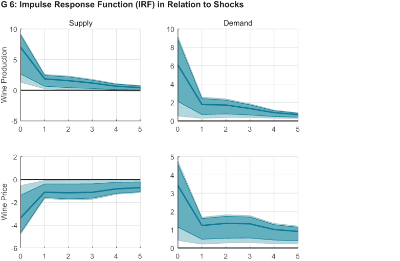
Thanks to the introduction of a theoretical impetus into the system, it is possible to analyse the response in terms of quantities and prices to supply-side or demand-side shocks. The two types of shock can be distinguished from each other by considering whether the trends are positive or negative: where quantity and price both evolve in the same direction (both positive, or both negative), a demand-side shock may be identified, whilst where they evolve in opposite directions (positive-negative or negative-positive) this will indicate a supply-side shock.
In the event of a positive supply-side shock (G 6: Supply), the quantity of wines increases by around 7 per cent compared to the reference level whilst the price falls by around 3 per cent. After the quantities return to equilibrium (after 5 months), prices are still affected (-1.5 per cent). In the event of a positive demand-side shock (G 6: Demand), the quantity rises by around 6 per cent compared to the reference level whilst the price increases by around 3.5 per cent. Although the quantity stabilises again after 5 months, the effect on prices is still felt for much longer.
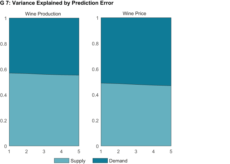
Graph G 7 displays the explained share of prediction error for each shock, respectively supply-side and demand-side, in relation to the two principal variables: quantity (left) and price (right).
Generally speaking, the quantity of wine appears to be more influenced by supply-side shocks, whilst the price of wine remains more balanced between the two types of shock. Over the long term, i.e. 5 months after the simulated a shock, demand appears to be of greater significance in interpreting variance explained in terms of both quantity and price.
Contact
No database information available